Scraping legislation to analyse changes over time

Introduction

Laws change over time. Governments frequently amend legislation and it can be hard to keep track of what has changed and when. The current verison of a given law shows traces of these changes, for example by mentioning how certain sections of other legislation have been repealed or amended by it. But it’s often hard to figure out how the substance of what has changed about a given law and when that change was made.

This is part 1 in a series of posts describing how to analyze the evolution of laws over time. It describes one way to use basic webscraping techniques to collect different versions of the same law. It uses Canada’s Immigration and Refugee Protection Act (IRPA) 2002 as an example. The post assumes that users have a basic functional knowlege of the R programming language as well as a high level understanding of HTML and CSS (mostly just a loose understanding of what they are).

Scraping historical versions of legislation

The first thing we will do is find a way to efficiently collect different versions of the legislation across time. Thankfully these legislative ‘snapshots’ are easy to find on Canada’s Justice Laws Website. Other countries like the UK and Australia also publish historical versions of legislation. All historical versions of the IRPA are conveniently linked at this URL: https://laws.justice.gc.ca/eng/acts/i-2.5/PITIndex.html.

Before we can scrape anything, we need to load the proper packages and define what’s called a user agent. User agents are basically a way to tell the page you’re scraping who you are.

### load necessary dependencies for project
pacman::p_load(tidyverse, rvest, httr)

#define user agent information for scrape
ua <-  user_agent("Mozilla/5.0 (Macintosh; Intel Mac OS X 13_1) AppleWebKit/537.36 (KHTML, like Gecko) Chrome/109.0.0.0 Safari/537.36")

Now we are ready to begin scraping. We can use our URL with the links to conduct what is called an index scrape. This just means we are collecting a list of URLs that point to the content that we are really after – text from different versions of the IRPA.

#this is our the url with the list
url <- "https://laws.justice.gc.ca/eng/acts/i-2.5/PITIndex.html"

Before we can extract our index from this URL, we need to figure out how the links to our content are embedded in the website. We just navigate to the url by pasting it into an internet browser or using browseURL(url) in our R console. We will use a browser plug in called Selector Gadget to select parts of the site we are interested in. There is a full tutorial on SelectorGadget.com but our use case is pretty straight forward. We just click on elements until the parts we want are highlighted in green or yellow. Parts we don’t want should be highlighted in red or not at all. Once satisfied with our selection, we copy the CSS selectors indicated in the bar on the bottom right of the page. In this case we want HTML nodes labelled as .col-md-push-3 a.

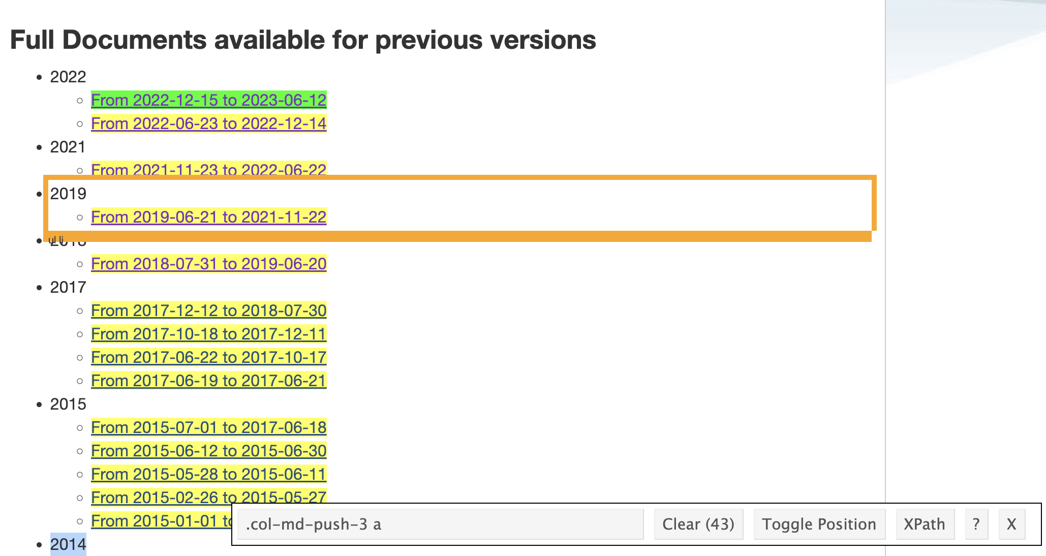This screenshot shows what it will look like with all of the appropriate links selected.

Now we are ready to scrape! The code chunk below uses the rvest package to read the HTML at our URL, select the parts we chose using Selector Gadget, and extract the embedded links. Because the links point to different parts of the same website, they only return the end of the URL. We need to complete the URLs by adding https://laws.justice.gc.ca/eng/acts/i-2.5/ to the start of them.

index <- read_html(session(url, ua)) |> #reads the HTML from the URL
  html_nodes(".col-md-push-3 a") |> #selects parts labeled with the CSS tag we identified with selector gadget
  html_attr("href") |> #extracts the 'href' HTML attribute (which means embedded URLS!)
  map_chr(\(x){paste0("https://laws.justice.gc.ca/eng/acts/i-2.5/", x)}) #complete the URLs

After we run this code, we should end up with an index – a list of URLS in our R environment. We can test that this worked by visiting some of the pages. For example browseURL(index[10]) for the 10th URL in our list. Once satisfied, we can begin to scrape the text. The code chunk below is even simpler than our index scrape. We read the HTML for each URL in the index and extract the text from it. We end up with 43 character strings in an element called text, each containing a different version of the IRPA.

text <- map(index, \(x){ #For each URL in index
    read_html(session(x, ua)) |> #read the HTML
    html_text2()}) |> #extract the text
  unlist() #unlist the mapped output

Getting metadata and managing our files

Now we will save this content in a way that will make it easy for us to use it in further analyses by saving a table with all of our texts and the URLs we took them from, writing each text entry to it’s own .txt file, and creating metadata for each text so we can keep track of all our files.

First, we create a table with columns for our text and the index URL that we took it from. We create a date variable which we can extract from each of the texts. Each text contains a string like this: “Version of document from 2022-12-15 to 2023-06-12”. So we can use the regular expression (?<=document from ).+(?= to) to extract the start date for each piece of legislation. We also format this as YYYY-MM-DD. We also create a variable with a file name that we will write the text to in the next stage. I want to write each version of the IRPA to a .txt file in a folder called ‘corpus’, so each name entry will look something like this: corpus/ca-irpa-2022-06-23.txt. Finally, we write our table to a .csv file called ca-irpa-versions.csv.

name <- tibble(text = text, index = index) |> # create a table with text and index as columns
  mutate(date = as.Date(str_extract(text, "(?<=document from ).+(?= to)"), "%Y-%m-%d"), # create a date variable by extracting and formatting the start date date from the text 
         name = paste0("corpus/ca-irpa-", date, ".txt"), #create file names
         doc_id = row_number()) |> #assign the rownumber as a unique doc_id
  write_csv("data/ca-irpa-versions.csv") #write to a .csv

You need to create a sub-directory called ‘data’ within the working directory for this code to run.

Now we will use this table to help us write each version of the legislation to its own text file. As text data can take up quite a bit of memory, it is good practice to clear your environment periodically. Now that we have a fresh start, we read in the table we create in the previous step, select the text and name columns, and then write each row of the table to individual .txt files. The text column is the content of each file and the name column is the file name.

rm(list = ls()) #clear the environment

read_csv("data/ca-irpa-versions.csv") |> #
  select(text, name) |> #select just the text and the file name
  pwalk(~ write_lines(x = .x, file = .y)) #along the text variable (.x), write the text to a file named according to the name variable (.y)

You need to create a sub-directory called ‘corpus’ within the working directory for this code to run.

Conclusion

This is where we will end with Part 1. If you followed along with this post you should now have:

1. A .csv file with the text of each version of the IRPA, the url that points to each version, the date that each version came into effect, and a column with a local path to a .txt file.
2. A folder called ‘corpus’ (or whatever else you decided to call it) with a .txt file for each version of the IRPA

In Part 2, we will use these files to begin analyzing how the IRPA has changed in the 2 decades since it was passed into law.