Cleaning legislation for computational analysis

Introduction

My last post used the example of Canada’s Immigration and Refugee Protection Act (IRPA) to show how to scrape different versions of legislative texts. For my research, I went ahead and scraped the versions of core immigration legislation for several countries. Before I can continue analyzing how these laws have evolved over time, I still need to clean up the text data that I scraped to ensure that I am only working with content that is relevant to my research question. In this case, I just want the text of the law and not the notes that are often embedded in legislation with editorial comments, lists of amendments, blank spaces for sections that have been repealed, and so on.

In this post, I use the example of the United Kingdom’s Immigration Act (1971) to show how to clean legislative text data. I am using this text instead of the IRPA because it was more complicated to clean up so is better for demonstrating some of the challenges that come up when working with legislative texts. As in part one, I assume that readers have a basic functional knowledge of the R programming language.

First thing’s first, we have to set up our file. We read in packages we’ll be using as well as the data. When I scraped the legislation, I created a .csv with four columns: $text with the content of the legislation; $index with the url it was scraped from, the $date of the version, and $name with a file name and local path to a .txt file. While the UK published versions going all the way to the 1970’s, I’ve applied a filter to remove versions from before the year 2000.

pacman::p_load(tidyverse)

uk <- read_csv('data/leg-versions/uk-imm-act-1971-versions.csv') |> #read in the data
  filter(year(date) >= 2000) |> #filter out years before 2000

Understanding the structure of the text

After reading in and filtering our data, we can take a closer look at the texts we are going to clean. Our primary questions at this stage are: What content are we interested in? What content is not needed? What patterns are apparent in how this content is structured?

We can investigate these questions in a couple of ways. First, we create a .txt file in our working directory of the most recent version in the console with this line:uk$text[93] |> write_lines('uk93.txt'). This text file is a good reference but I also like to pull up the web version of the document I am working with.

The screenshot below shows us the first several lines of the Immigration Act and we can see right away that the text of the law (which begins with the line “An Act…”) is accompanied by supplementary notes about amendments contained in the box with the heading “Modifications etc.”. We can note, for example that many of the lines in the box start with ‘C’ followed by a number. We can also see that each line begins with “Act” followed by one of several verbs like “amended” or “modified”. Many of these lines include references to other laws using a codified shorthand with repeated patterns like “c.” and a number (“c. 33”), references to a section (“s. 59”), sections (“ss. 69”) or schedule (“Sch. 2”). A quick search using Ctrl-F reveals this shorthand only appears in the boxes with notes, while the text of the legislation will spell out ‘section’ or ‘schedule’ when referring to these things. We will keep these notes in mind.

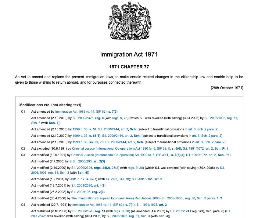This screenshot shows the first lines of the most recent version of the UK’s Immigration Act 1971 with LOTS of text that we don’t want or need for our analysis.

Despite discovering a really useful set of patterns in the text of the most recent version of the legislation, there is no guarantee these patterns will hold in older versions. Let’s go to the opposite extreme and look at the oldest version we have. Again we can write a .txt file to look at the raw text we scraped using this line: uk$text[1] |> write_lines('uk1.txt'). We can also look at the first web version of the law from 2000.

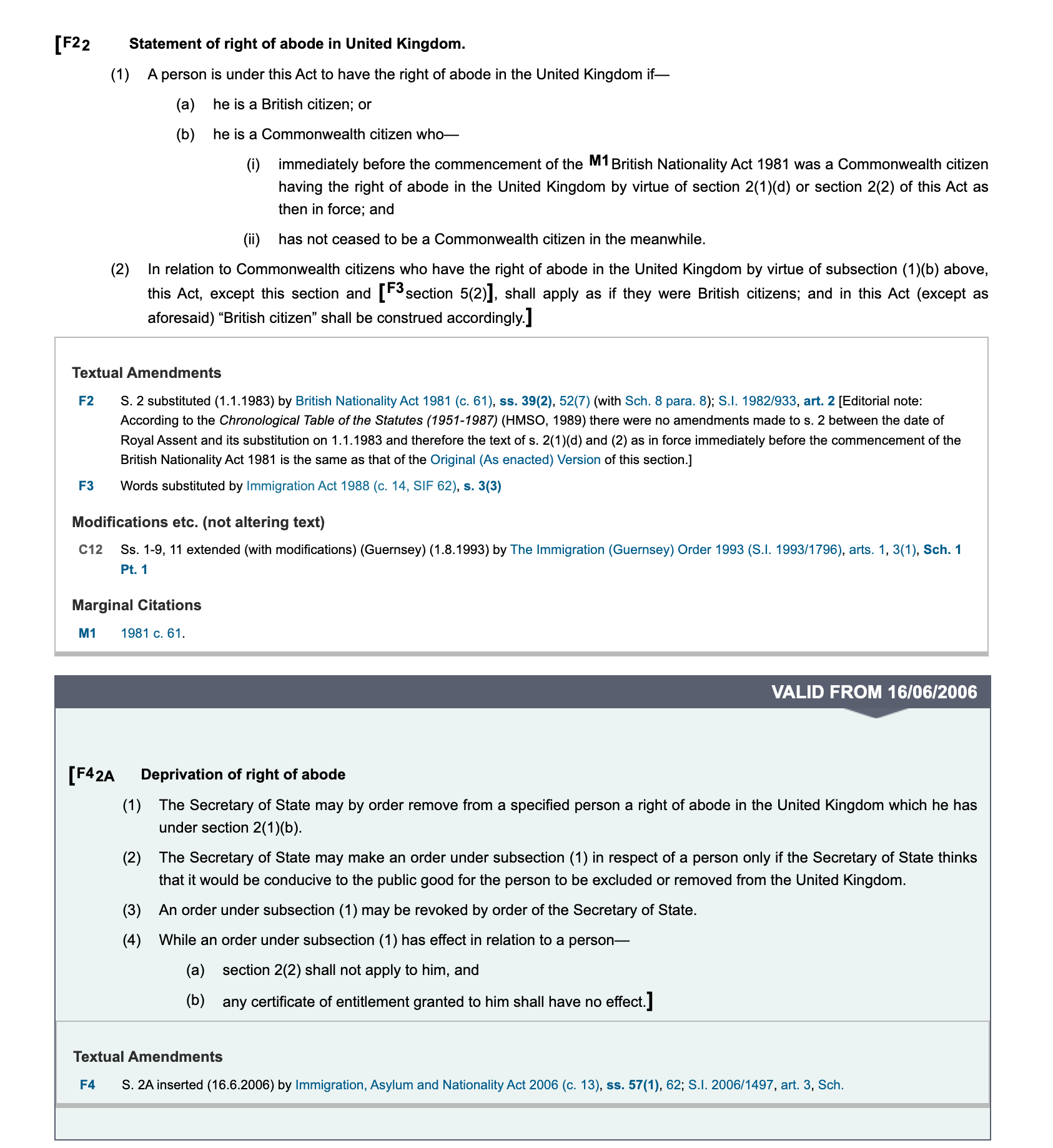This screenshot of the earliest piece of legislation in our series reveals additional editorial notes that we don’t need.

Looking at the published version from February 14th, 2000 reveals additional editorial content that we need to remove. First, we see that amendments are referenced in the text using square brackets – this appears in all versions of the legislation but I’m noting it here because it appears in this screenshot. What isn’t in the latest version is the box that shows future amendments. In this case we have a box that starts with “VALID FROM” followed by a date in DD/MM/YYYY format. It ends with the standard notation for the textual amendment we already identified. Another quick search using Ctrl-F shows that this pattern holds for all of these boxes.

These are some of the most important examples, but I spent a fair bit of time examining different versions of the legislation to identify these sorts of patterns and test them for consistency. The next section of this post will go over how I translated these patterns into a series of regular expressions to extract the parts of the UK’s Immigration Act 1971 that I’m interested in and remove those that are not going to be helpful for my next stage of analysis.

Using and applying regular expressions

Regular expressions are patterns used to match character combinations in strings. They are crucial for cleaning textual data. My cleaning process for legislation scraped from the internet is broken into two stages. In the first step I use dplyr::mutate() and stringr::str_remove_all() to remove all text in each row of our data frame between “Valid from” and “Textual amendments”.

uk <- uk |>
  mutate(text = str_remove_all(text, "Valid from[\\s\\S]+?(?=Textual Amendments)"), #remove all content between "Valid from" and "Textual amendments"

Let’s break down the expression used:

"Valid from" matches that exact sequence of characters. [\\s\\S] matches any character:

• \\s: Matches any whitespace character, which includes spaces, tabs, and line breaks.
• \\S: Matches any non-whitespace character. By combining them within the square brackets [...], we’re basically creating a pattern that can match any character, be it whitespace or not. +? modifies the preceding pattern ([\\s\\S]).
• +: Matches one or more of the preceding element.
• ?: Makes the + “lazy”, meaning it will try to match as few characters as possible. Without the ?, the + would be “greedy” and would try to match as many characters as possible.

(?=Textual Amendments) is a positive lookahead assertion that matches the exact string inside of the brackets.

• (?=...): This will look ahead to see if there’s a match, but won’t consume any characters. In this case, it’s looking to see if “Textual Amendments” follows after the earlier matched sequence. If “Textual Amendments” does not follow, then the whole regular expression won’t match.

Basically, this regular expression will find and match the sequence “Valid from” followed by any number of characters (as few as possible) until it matches “Textual Amendments”, without including “Textual Amendments” in the match itself.

The second step uses a ‘for loop’ to iterate over each version of legislation, transforming each version into a tibble (a dataframe format used in tidyverse) with a row for every line in the text of the legislation.

Many experienced R programmers dislike ‘for loops’. Their reservations are generally well founded. For loops are computationally inefficient and less legible than ‘vectorized’ approaches like purrr::map(), especially for more complex tasks. For our purposes the task is small and simple enough that a for loop is fine.

for(i in 1:length(uk$name)){ #for each file in the UK CSV
  tibble(text = read_lines(uk$text[i])) |> #read each line as a row in a spreadsheet
    filter(#remove rows that begin with these patterns (indicating the notation describing amendments)
      !str_detect(text, " s\\.| S\\.| Sch\\.| ss\\.|\\dS\\."),
      !str_detect(text, "(. . . . )+"),
      !str_detect(text, "^C\\d+|^I\\d+|^M\\d+"),
      !str_detect(text, "Textual Amendments|Modifications etc|Commencement Information|Marginal Citations")) |>
    #remove text (not full rows) that matches the following strings
    mutate(text = str_remove_all(text, "\\[F\\d+"),
           text = str_remove_all(text, "F\\d+\\["),
           text = str_replace_all(text, '\\]', ' '),
           text = str_remove_all(text, "F\\d+"),
           text = str_remove_all(text, "U\\.K\\."),
           text = str_remove_all(text, "M\\d+"),
           text = str_remove_all(text, "\\([\\s\\S]{1,4}\\)"),
           text = str_remove_all(text, "\\d+"),
           text = str_remove_all(text, "PART"),
           text = str_replace_all(text, "\\b[A-Z]+([A-Z][a-z]+)\\b", "\\1"),
           text = str_squish(text)) |> #delete extra spaces
    head(-2) |> 
    filter(!text == "", #remove empty rows
           !text == " ") |> 
    write_delim(uk$name[i], delim = "\r", col_names = FALSE) #write to a .txt file in the UK folder
  
  print(paste("Finished", uk$name[i])) #print the file name of each file one it have been processed
}

The code works as follows: The loop iterates over each file name in the uk dataframe. This reads each line of the file referenced by uk$text[i] into a tibble. It then uses dplyr::filter()and several regular expressions to remove rows that meet the following conditions:

• Rows that start with notations indicating amendments.
• Rows with repeated periods, which indicate repealed text.
• Rows that start with codes like “C12”, “I5”, etc.
• Rows containing certain specific phrases, such as “Textual Amendments” and “Marginal Citations”, which are standard headers for editorial notations.

It then uses dplyr::mutate() to modify and remove specific text from the rows as well (without deleting the entire row as above):

• Removing patterns that point to footnotes or references, such as [F1] or F1[.
• Replacing closing brackets (]) with spaces.
• Removing certain patterns and abbreviations like “U.K.”, which appears throughout the scraped content as a ‘tag’.
• Removing references that are surrounded by parentheses and are up to 4 characters long, like (A) or (iv).
• Removing all numbers.
• Removing the word “PART”.
• Replacing words starting with multiple capital letters (like “AExample”) to start from the last capital letter (like “Example”).
• Using str_squish() to collapse and remove any extra whitespace.

We then use head(-2) to remove the last two lines – extraneous formatting from the website and then filter again to remove any empty rows created by multiple line breaks in the original text and in cases where we removed all the content in a row in the steps above. Finally, we use write_delim() to put each row in the tibble into a line in a .txt file written to the local path in our original .csv file. The final part of our for loop prints the name of the file that has just been processed so if there is an error we can see which file caused the problem.

Validating the outputs

Now that we have applied our cleaning script to every version of the legislation, we should take steps to validate the process. In this case I used the diffr library to compare the text before and after applying this process.

We start by create a subset of the versions we cleaned by filtering the the scraped text to versions after the year 2000 and then extracting the oldest and the most recent versions. Then we take the ‘raw’ text from our scrape and write two .txt files in a subdirectory I created called data/validate.

# Load the UK immigration act versions from a CSV file. 
uk_sub <- read_csv('data/leg-versions/uk-imm-act-1971-versions.csv') |> 
# Filter rows where the year is 2000 or later. 
filter(year(date) >= 2000) |> 
# Filter to get only the rows with the earliest and latest dates. 
filter(date == min(date) | date == max(date))

# Modify the file paths and write the text data to new files.
uk_sub |> 
# Update the directory paths in the 'name' column. 
mutate(name = str_replace(name, "corpus/uk/", "data/validate/raw-")) |> 
# Select only the 'text' and 'name' columns. 
select(text, name) |> 
# For each row, write the text to the specified file. 
pwalk(~write_lines(x = .x, file = .y))

Next we use list.files() to put the paths to the two files we just wrote in a vector called raw. We put the paths from our subset, which point to the .txt files we wrote during our cleaning process in a vector called clean. Both vectors are sorted so that the file names appear in the same order.

# List all files in the 'data/validate' directory with names starting with 'raw-uk' and sort them. 
raw <- list.files('data/validate', pattern = "raw-uk", full.names = TRUE) |> sort() 
# Sort the names in the 'uk_sub' data frame. 
clean <- uk_sub$name |> sort()

Finally, we use a for loop to feed the raw and cleaned text of the oldest and newest versions of the UK Immigration Act to a function called diffr, which compares the two versions of each text and highlights differences between them by presenting them to us side-by-side in an .html file. “Diffing” is a common method used to view changes in computer code across different versions but it’s a handy tool for these purposes too!

# Loop to compare and generate differences between the raw and cleaned files. 
for(i in 1:2){ 
# Compare the files and save the differences as an HTML widget. 
diffr(raw[i], clean[i]) |> htmlwidgets::saveWidget('tmp.html', selfcontained = TRUE) 
# Rename 'tmp.html' using the base file names indicated in the metadata. 
file.rename("tmp.html", paste0("data/validate/html/", str_extract(raw[i], "(?<=validate/raw-).+(?=\\.txt)"),".html")) }

The code used above fed us two .html files that we can open in a web browser to manually verify that our function has removed the content we want gone without accidentally removing content we need.

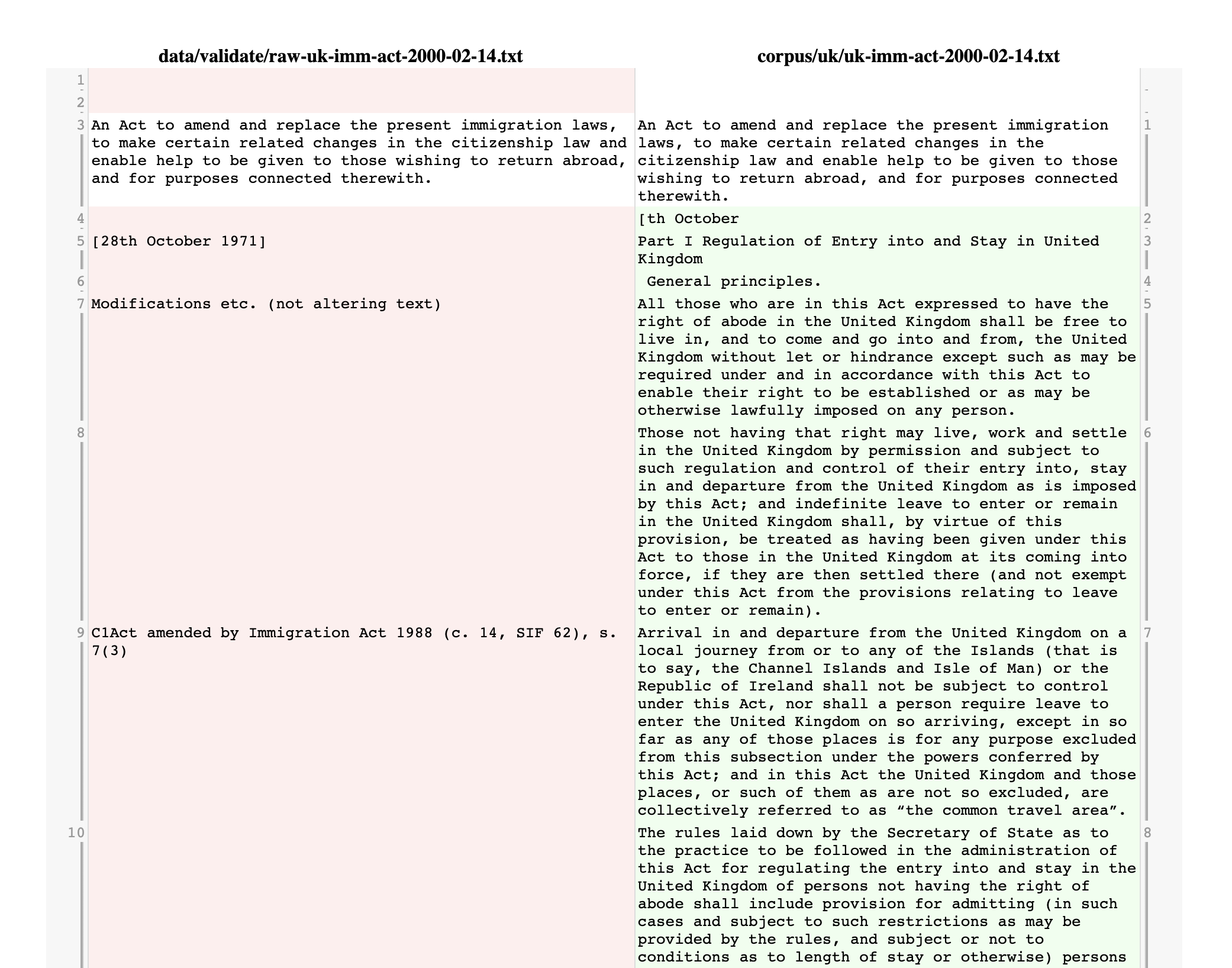This screenshot shows what one of the diffr .html files looks like

We can open up the .html file in our browser and scroll through. As we can see in the screen shot above our cleaning has removes a lot of extra white space as well as needless formatting, numbers and editorial notes. It takes a while to scroll through them but it’s worth it as I caught several mistakes throughout my cleaning process. For this example, I am using the oldest and newest versions, which was my starting point. In practice, validation was an iterative process where I consulted several different versions (including those in the middle of the date range) throughout the cleaning process.

This post is linear but the cleaning process was not! I validated my cleaning as I was writing the code, going back and forth several times to get the final result. The final result is not perfect. The text will still need to be pre-processed before I can apply computational methods like topic models. Because different methods call for different pre-processing, this is a convenient way to store it for now.

Conclusion

This is where I’ll stop with part 2 of this series on analyzing how legislation evolves. Admittedly, this post was not a full service tutorial as you would have had to scrape the legislation or use the Canadian legislation scraped in part 1. But if you followed along, you should have a folder of .txt files containing the cleaned text of each version. You’ll also have at least two .html files displaying the differences between the ‘raw’ and cleaned text. In future posts we will read these texts into a corpus that we can pre-process and apply various computational methods.